Let’s start with the best tutorials for deep learning and CNNs.
- Genreal Tutorials:
- An Intuitive Explanation of Convolutional Neural Networks by Ujjwal Karn
- Unsupervised Feature Learning & Deep Learning Tutorial by Andrew NG
- CS231n Convolutional Neural Network for Visual Recognition by Feifei Li
- Deep Learning Tutorial by Theano Development Team
- Classic Papers:
- AlexNet by Alex Krizhevsky, Ilya Sutskever& Geoffrey Hinton from University of Toronto
- VGG: Very Deep Convolutional Neural Networks for Large-Scale Image Recognition by Visual Geometry Group, University of Oxford
- GoogLeNet: Going Deeper with Convolutions by Google Inc
- ResNet: Deep Residual Learning for Image Recognition by Microsoft
AlexNet
Adit has a good summary of its importance:
The one that started it all.
2012 marked the first year where a CNN was used to achieve a top 5 test error rate of 15.4% (Top 5 error is the rate at which, given an image, the model does not output the correct label with its top 5 predictions). The next best entry achieved an error of 26.2%, which was an astounding improvement that pretty much shocked the computer vision community. Safe to say, CNNs became household names in the competition from then on out.
Statistics
- Year: 2012
- Data: 1.2 million images from ImageNet LSVRC-2010
| Top 1 Error | Top 5 Error | |
|---|---|---|
| AlexNet | 37.5% | 17.0% |
Architecture
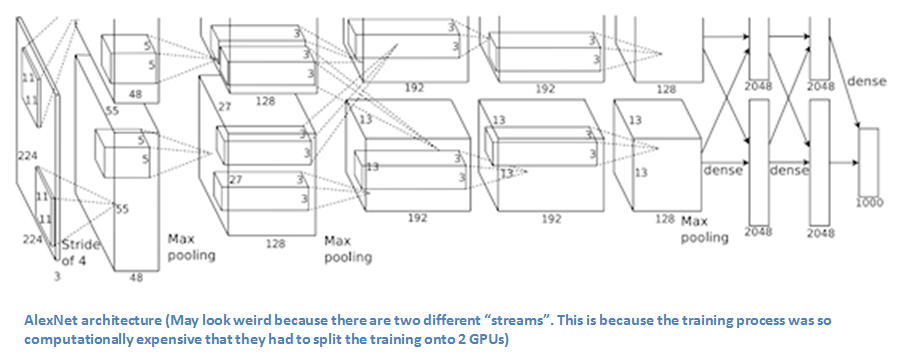
| Layers | Remarks | |
|---|---|---|
| 1 | Convolutional: 96 kernels of 11*11*3, stride 4 | response normalized & pooled |
| 2 | Convolutional: 256 kernels of 5*5*48 | response normalized & pooled |
| 3 | Convolutional: 384 kernels of 3*3*256 | |
| 4 | Convolutional: 384 kernels of 3*3*192 | |
| 5 | Convolutional: 256 kernels of 3*3*192 | |
| 6 | Fully connected: 4096 neurons | |
| 7 | Fully connected: 4096 neurons | |
| 8 | Fully connected: 4096 neurons | |
| Output layers: 1000, softmax |
Note that, later in the more successful version ZF Net, the size of kernel is modified from 11*11*3 to 7*7*3 to capture more details in the image.
- training schema
We use stochastic gradient descent with a batch size of 128 examples, momentum of 0.9, and weight decay of 0.0005.
We initialized the weights in each layer from a zero-mean Gaussian distribution with standard deviation 0.01. We initialized the neuron biases in the second, fourth, and fifth convolutional layers, as well as in the fully-connected hidden layers, with the constant 1. This initialization accelerates the early stages of learning by providing the ReLUs with positive inputs. We initialized the neuron biases in the remaining layers with the constant 0.
Main Take-aways
| Save Time | Increase Accuracy | Reduce Overfitting | |
|---|---|---|---|
| ReLU | 6 times faster than Tahn/ Sigmoid activations | ||
| Multiple GPUs | ☑️ | ||
| Drop Out layer | 1/2 of time required to converge | ☑️ | |
| Local Response Normalization | Top1: 1.4%; Top5: 1.2% | ||
| Overlapping Pooling | Top1: 0.4%; Top5: 0.3% | ||
| Data Augmentation | ☑️ |
Data Augmentation Methodologies
Extracting random 224 × 224 patches (and their horizontal reflections) from the 256×256 images and training our network on these extracted patches 4.
Altering the intensities of the RGB channels in training images…. We perform PCA on the set of RGB pixel values, To each training image, we add multiples of the found principal components, with magnitudes proportional to the corresponding eigenvalues times a random variable drawn from a Gaussian with mean zero and standard deviation 0.1.
VGG
VGG is the first paper that discusses about the depth of CNN architecture. It extends the number of layers to 19 and uses very small (3*3) convolutional filters. It also states that VGG model could be used as a part in other machine learning pipeline as deep features.
Statistics
- Year: 2014
- Data: 1.3 million images from ImageNet ILSVRC-2012
| Top 1 Error | Top 5 Error | |
|---|---|---|
| AlexNet | 37.5% | 17.0% |
| VGG | 23.7% | 7.3% |
Architecture
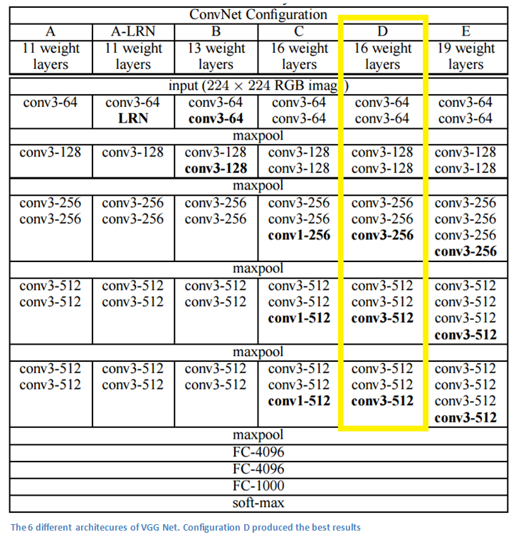
Note that, All hidden layers are equipped with the rectification (ReLU (Krizhevsky et al., 2012)) non-linearity. the ReLU activation function is not shown for brevity.
- Changes from AlexNet
| AlexNet | VGG | |
|---|---|---|
| Layers | 5 Conv, 3 FC layers | 16 Conv, 3 FC layers |
| Convolutional Filters | 11*11; stride = 4 | a stack of conv layers with 3*3 kernels, stide =1 |
| Padding | None | 1 |
| Pooling | Overlapping Max Pooling | Non-overlapping Max Pooling |
| Local Response Normalization | Yes - it improves performance | No - it doesn’t improve performance but increase memory & computation time |
- Training Schema
| AlexNet | VGG | |
|---|---|---|
| Batch size | 128 | 256 |
| Momentum | 0.9 | 0.9 |
| Weight decay | 0.0005 | 0.0005 |
| Initialization | N(0,0.01); bias = 1 | N(0,0.01); bias = 0 |
Main Take-aways
Deep CNN!
Why would we use stack of multiple 3*3 Convolutional layers (without spatial pooling in between) instead of larger one layer kernel?
Same receptive filed.
Receptive filed is well explained by Novel Martis in this post. For example, in the below image, the input for B(2,2) is A(1:3, 1:3). The input for C(3,3) is B(2:4, 2:4) -> A(1:5,1:5). The receptive field for 2 convolutional layers will be 5*5, and 3 convolutional layers will be 7*7.
More discriminative function.
There are three ReLU layers instead of one.
Less parameters.
Suppose we have C channels. Stack of three 3*3 kernels will have 3(3^2) = 27 parameters, and one layer of 7\7 kernel will have 7^2 = 49 parameters; which is 81% more.
Inception
Inception goes beyond the idea “we need to go deeper” but comes up with a “network-in-network” inception module. There are two drawbacks of the previous most popular deeper and wider neural network - that it might easily go overfitting especially when there’re no enough training examples, and that it takes up too much computational resources. The authors are motivated to build more efficient yet accurate (or more accurate) algorithms by replacing the fully connected layers with dense structures.
Statistics
Year: 2015
Data: 1.3 million images from ImageNet ILSVRC 2014
| Top 1 Error | Top 5 Error | |
|---|---|---|
| VGG | 23.7% | 7.3% |
| Inception | 6.7% |
Architecture
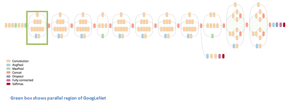
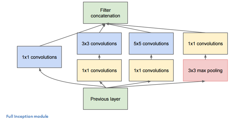
Inception Module:
So the green box above is an inception module, which could be presented as the picture below. The idea behind is that the authors try to find a dense structure that can best approximate the optimal local sparse structure. So the idea is well outlined in Adit’s blog: previously in stacked CNNs, different sizes of convolutional layers and max pooling layers are to be chosen; here we have them all. For example, if inside one picture, there is a person stands nearer the camera while there is a cat that is far away from the camera, it would be beneficial to have both of a larger image kernel to capture the nearer person and a smaller kernel to capture the cat. Therefore with the inception module, parameters are less, yet more powerful than simply stacked convolution.
Main Take-Aways
The idea of CNN doesn’t have to be stacked up sequentially.
Get rid of fully connected layer (use average pooling instead) thus saves a lot of parameters and computational time.
The massive usage of 1*1 convoluational kernel:
Dimensional reduction
The 1*1 kernel is reducing a great amount of image dimensions. For example, if there is 224*224*60 input that goes through a 1*1*10 image kernel, then the output size will just be 224*224*10.
Less parameters, less chance of overfitting
ResNet
ResNet aims to solve the problem of degradation.
Basically, the authors of ReNet found that with increased number of layers, the accuracy get saturated thus degradation occurs. Previously the degragation was thought to be overfitting, but it isn’t: The training error increase rather than decrease. This is counterintuitive. The authors believe that, “the degradation problem (of training accuracy) suggests that the solvers might have difficulties in approximating identity mappings by multiple nonlinear layers.” Therefore he is motivated to create an easier way to optimize the deep CNNs.
Statistics
Year: 2015
Data: ILSVRC 2015
| Top 5 Error | |
|---|---|
| Inception | 6.7% |
| ResNet | 3.6% beats human recognition: 5%-10% |
Architecture
Residual Block
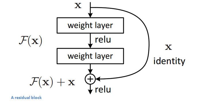
It performs shortcut identity mapping. I will reference Adit’s wonderful explanation here:
The idea behind a residual block is that you have your input x go through conv-relu-conv series. This will give you some F(x). That result is then added to the original input x. Let’s call that H(x) = F(x) + x. In traditional CNNs, your H(x) would just be equal to F(x) right? So, instead of just computing that transformation (straight from x to F(x)), we’re computing the term that you have to add, F(x), to your input, x. Basically, the mini module shown below is computing a “delta” or a slight change to the original input x to get a slightly altered representation (When we think of traditional CNNs, we go from x to F(x) which is a completely new representation that doesn’t keep any information about the original x). The authors believe that “it is easier to optimize the residual mapping than to optimize the original, unreferenced mapping”.
Another reason for why this residual block might be effective is that during the backward pass of backpropagation, the gradient will flow easily through the graph because we have addition operations, which distributes the gradient.
Reference
- The 9 Deep Learning Papers You Need to Know About
- An Intuitive Explanation of Convolutional Neural Networks
- CS231n Convolutional Neural Network for Visual Recognition by Feifei Li
- AlexNet by Alex Krizhevsky, Ilya Sutskever& Geoffrey Hinton from University of Toronto
- VGG: Very Deep Convolutional Neural Networks for Large-Scale Image Recognition by Visual Geometry Group, University of Oxford
- GoogLeNet: Going Deeper with Convolutions by Google Inc
- ResNet: Deep Residual Learning for Image Recognition by Microsoft