This blog summarizes image processing methods from pyimagesearch. All the source codes and pictures come from the blog and I won’t take any credit for anything.
Image Processing
References
Codes
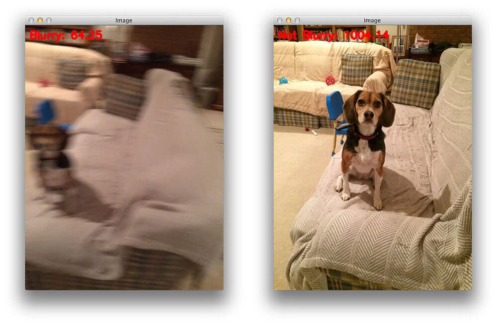
- Blur Detection
|
|
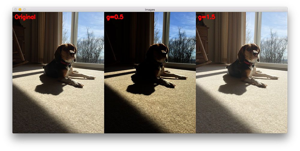
- Gamma Correction
|
|
Object Detection
References
Detecting Circles in Images using OpenCV and Hough Circles
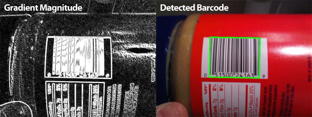
Detecting Barcodes in Images with Python and OpenCV
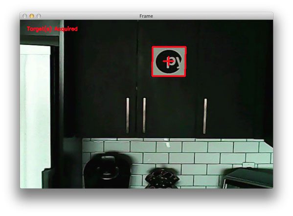
Target acquired: Finding targets in drone and quadcopter video streams using Python and OpenCV
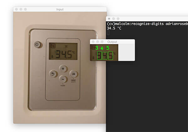
Recognizing digits with OpenCV and Python
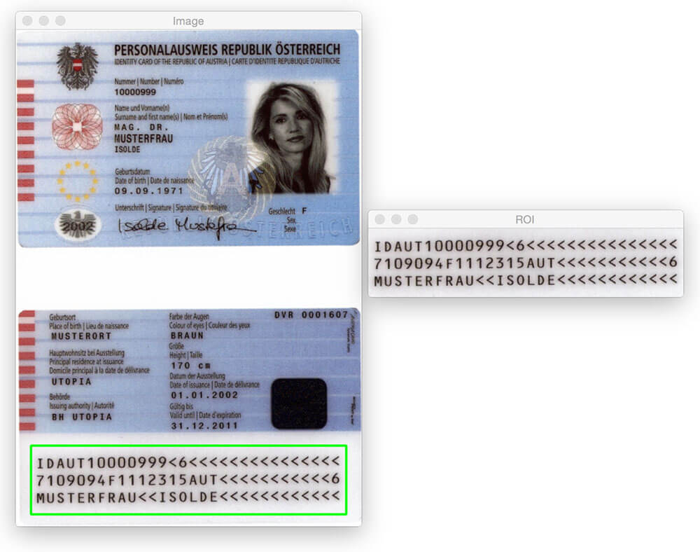
Detecting machine-readable zones in passport images
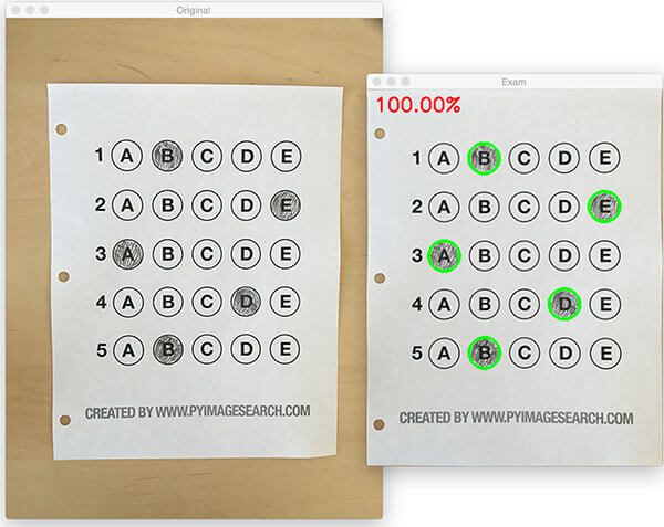
Bubble sheet multiple choice scanner and test grader using OMR, Python and OpenCV
Codes
- Detecting Circles
|
|
- Detect squares in a video
|
|
- Detectin Texture (Barcode in this case)
|
|
- Detect Digits Areas
|
|
- Detect Machine Readable Zones
|
|
Object Transformation
References
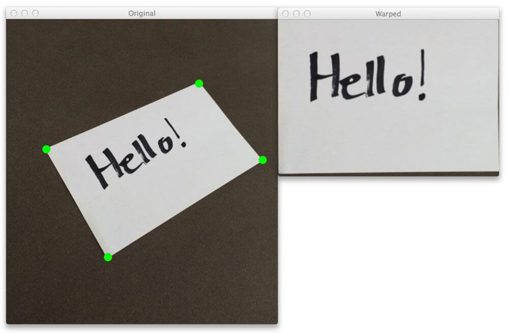
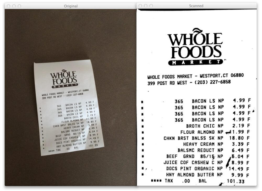
4 Point OpenCV getPerspective Transform Example
How to Build a Kick-Ass Mobile Document Scanner in Just 5 Minutes
Text skew correction with OpenCV and Python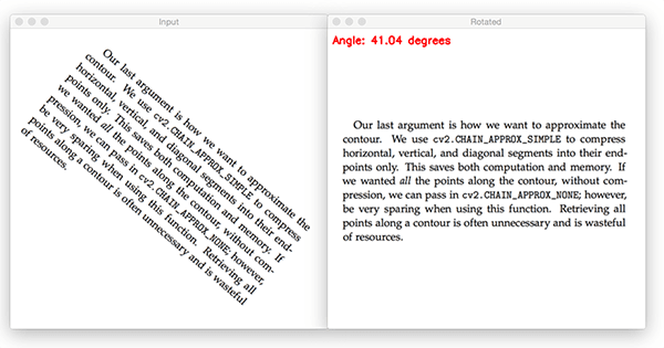
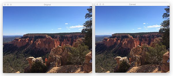
Seam carving with OpenCV, Python, and scikit-image
Codes
- Four Point Transformation
|
|
|
|
- Text Skew Correction
|
|
Template Matching
References
Multi-scale Template Matching using Python and OpenCV
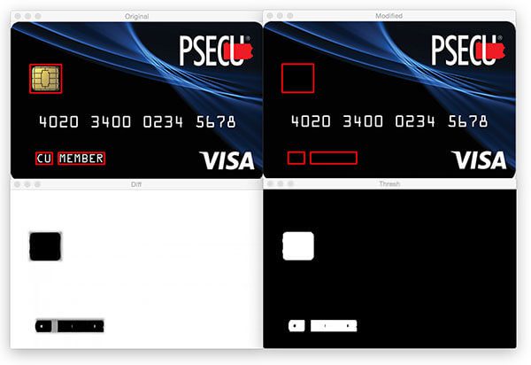
Image Difference with OpenCV and Python
Codes
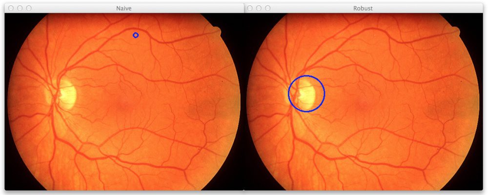
- Robust Template Matching
|
|
- Image Difference
|
|
Color Manipulation
References
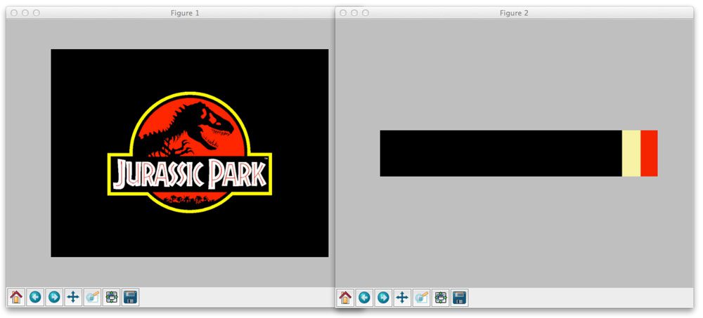
Finding the Brightest Spot in an Image using Python and OpenCV
OpenCV and Python K-Means Color Clustering
Color Quantization with OpenCV using K-Means Clustering
Codes
- Brightest color:
|
|
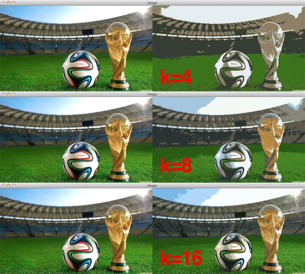
Color Quantization:
Color quantization limits the number of colors remained in one picture. For example if there is sky blue and dark blue, they might be combined into some color in the middle of their RGB value. It removes redundant color information thus saves storage spaces. It’s useful in image search problems.
|
|