Introduction
Kalman Filter, an artificial intelligence technology, has been widely applied in driverless car navigation and robotics. It works well in presence of uncertainty information in dynamic systems. It is a linear solution based on Bayesian Inference especially for state space models. – This is the definition in the hard way.
Lets skip the first paragraph and look at a little story.
Source: Kalman Filter: Theories and Applications
A group of young men were standing, under their feet there was a twisty narrow road to a very big tree. One man walked to the tree, asking, “can any of you walk to the tree with your eyes closed?”“That’s simple, I used to serve in the army.” Mike said. He closed his eyes and walked to the tree like a drunk man. “Well, maybe I haven’t practiced for long.” He murmured. - Depending on prediction power alone.
“Hey, I have GPS!!” David said. He held the GPS and closed his eyes, but he also walked like a drunk man. “That’s very bad GPS!” He shouted, “it’s not accurate!!” - Depending on measurement which has big noises
“Let me try.” Simon, who also served at the army before, grabbed the GPS and then walked to the tree with his eyes closed. - Depending on both of prediction power and measurement
After reaching the tree, he smiled and told everyone, “I am Kalman.”
In the story above, a good representation of the walking state at time k is the velocity and position.
$$ X_k = (p, v) $$
So there are two ways to measure where you are.
- you predict based on your own command system - it records every commands sent to you, but only some of commands are executed exactly as what they were - wheels may slip or wind may affect;
- you measure by your GPS system - it measures where you are based on satellite, but it can’t be as accurate as in meters and sometimes signals lost.
With Kalman Filter, we will get better understanding of where you are and how fast you go than either of the prediction or measurement. That is, we update our belief of where you are and how fast you go by incorporating the two sources of predictions and measurements using Bayesian inference.
Understanding Kalman Filter
Note: all the knowledge and photos for this section come from Ref 2. This is a study note only.
The whole idea of Kalman Filter can be represented by a single picture. It might look complicated at this moment, but we will understand everything after this article (if not, read Ref 2 - it’s a much nicer article I believe).
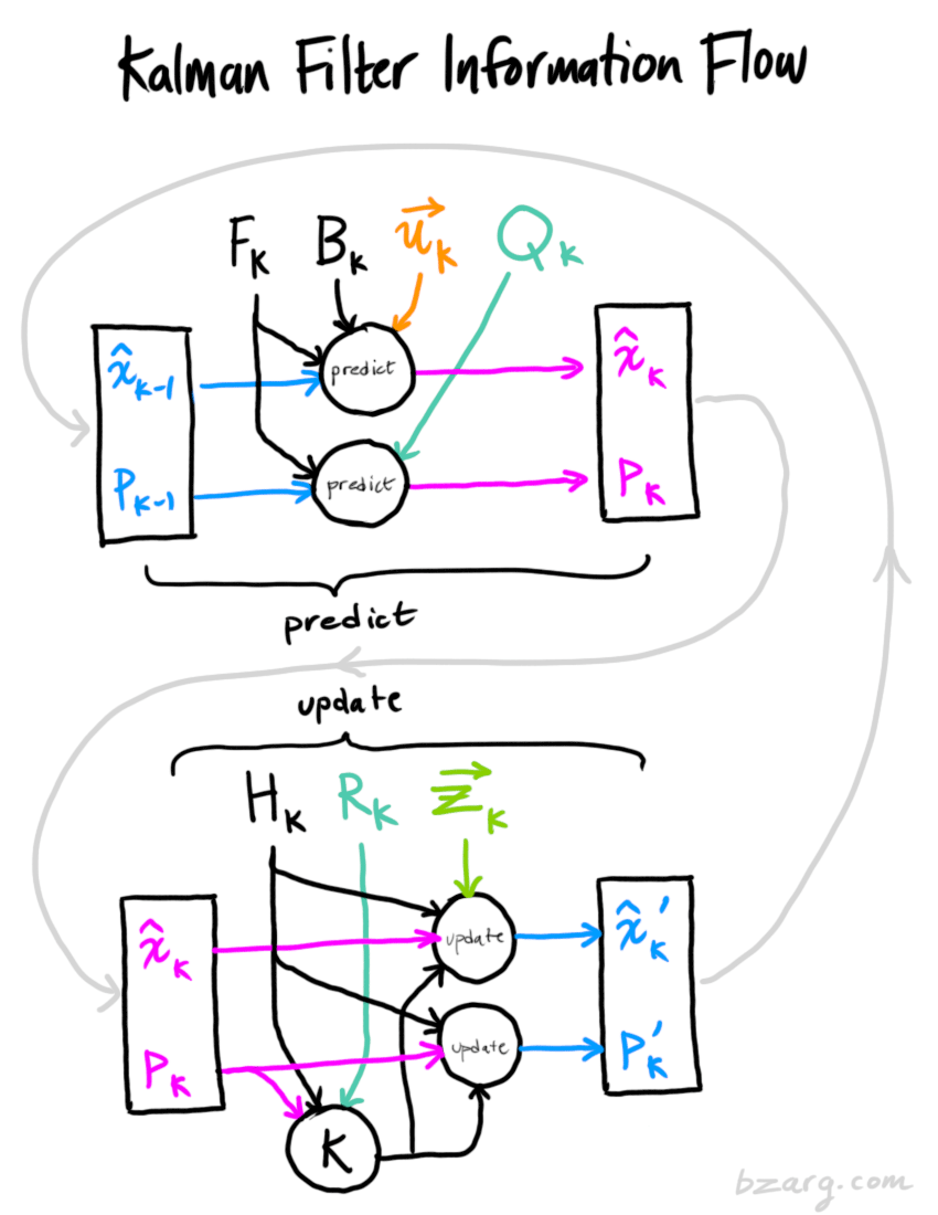
[source: ref 2]
Prediction Phase: $X_k, P_k, F_k$
$X_k$: Position and Velocity
Remember in our scenario, we want to know the position and velocity. We represent the state of the walking people at time k as $X_k = [position_k; velocity_k]$.
$F_k$: Prediction Matrix
We have
$ Position_k = Velocity_{k-1} * t + Position_{k-1} $
$ Velocity_k = Velocity_{k-1} $
The above two formulas could be written as:
$ \begin{bmatrix} Position_k \\ Velocity_k \end{bmatrix} = \begin{bmatrix} 1 & t \\ 0 & 1 \end{bmatrix} * \begin{bmatrix} Position_{k-1} \\ Velocity_{k-1} \end{bmatrix} $
We represent the prediction matrix $\begin{bmatrix} 1 & t \\ 0 & 1 \end{bmatrix} $ as $F_k$. We have then $ X_k = F_k * X_{k-1} $
$P_k$: Covariance Matrix
Since in our case, the faster the robot walks, the further the position might be. Therefore velocity and position should be correlated; the covariance matrix is $P_k$ .
When prediction matrix updates X_k, the change will also reflect on covariance matrix. Therefore $ P_k = F_k * P_{k-1} F_k^T $ .
Measurement Phase: $Z_k, H_k$
$H_k$: Measurement Function
Sometimes the GPS reading is not having the same units with the prediction states. For example, we use km/h in prediction states and we use m/s in GPS reading for velocity. So we need a transformation with matrix $H_k$:
$$ X_k = H_k X_k $$
$$ P_k = H_k P_kH_k^T $$
$Z_k$: Measurement
Remember the GPS reading is not very reliable and might have some variations. So it is represented as a Gaussian distribution with mean $Z_k = [PositionReading_k, VelocityReading_k]$. So in below picture the pink circle represents the prediction distribution while the green circle represents the measurement distribution. The bright bubble insight represents the belief distribution of position and velocity.
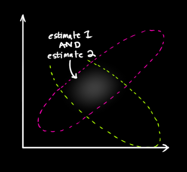
[source: ref 2]
External Factors: $R_k, Q_k, B_k, U_k $
$R_k, Q_k$: noises
$Q_k$ is the transition covariance for the prediction phase. $ P_k = F_kP_{k-1}F_k^T + Q_k $. The idea is that there would always be some uncertainty. Therefore we kept an assumption - points might move a bit outside its original path. In practice, the value is often set very slow, for example:
|
|
$R_k$ is the observation covariance for the measurement phase. $ P’_k = P’_{k-1} + R_k $. Default set as 1.
$B_k, U_k$: External influence
For example, if the people are going down from the mountain, he might walker quicker because of the gravity. Therefore we have
$$ Position_k = Velocity_{k-1} * t + Position_{k-1} + gt^2 /2 $$
$$ Velocity_k = Velocity_{k-1} + gt $$
Therefore we have
$$ X_k = F_k X_{k-1} + \begin{bmatrix} t^2/2 \\ t \end{bmatrix} g = F_k X_{k-1} + B_k U_k $$
where $ B_k $ is the control matrix for external influence and $U_k$ is the control vector.
The Big Boss: Kalman Gain ?
We are almost done explaining all the variables in Kalman Filter, except a very important term: Kalman Gain. This is a bit complicated, but luckily, this is not something we need to calculate or input.
Now let’s go back to the measurement phase once more. When we multiplying the prediction distribution and measurement distribution, the new mean and variance go like this:
$$ u’ = u_0 + \sigma_0^2 (u_1 - u_0)/ (\sigma_0^2 + \sigma_1^2) $$
$$ \sigma’^2 = \sigma_0^2 - \sigma_0^4/(\sigma_0^2 + \sigma_1^2) $$
so we make: $ k = \sigma_0^2/ (\sigma_0^2 + \sigma_1^2) $ where k is the kalman gain, therefore we can simplify the above equations to:
$$ u’ = u_0 + k(u_1 - u_0) $$
$$ \sigma’^2 = (1-k)\sigma_0^2 $$
Therefore Kalman gain helps updating the new $X_k, P_k$ value after seeing the measurement. So what is an intuitive explanation of Kalman Gain? It actually calculates the uncertainty in the prediction phase to the measurement phase, so it tells how much we should trust the measurement when updating $X_k, P_k$.
Python Implementation
I’d love to recommend a great post which gives applications of Kalman Filter in financial predictions with codes posted on its Jupyter Notebook. It demonstrates why we should use Kalman Filter comparing to linear regression just in one picture:
 [source: ref 3]
Parameter Mapping
Recall: Kalman Filter measures uncertain information in a dynamic systems. In this case, we want to know the hidden state slope and intercept. Let’s map all the inputs from theoretical to practical settings.
Prediction Phase
- State: $ X_k = \begin{bmatrix} \alpha_k \\ \beta_k \end{bmatrix} $
- Prediction Matrix: $ F_k = \begin{bmatrix} 1&0 \\ 0&1 \end{bmatrix} $.
This is because we assumes the slope and intercept aren’t correlated. - Intial State Covariance $ P_0 = \begin{bmatrix} 1 & 1 \\ 1 & 1 \end{bmatrix} $
Measurement Phase
- Measurement Function $ H_k = \begin{bmatrix}EWA & 1 \end{bmatrix} $.
The measurement we have is EWC. It’s obvious that it doesn’t share the same measuring units with slope and intercept. Since we have EWC = EWA*slope + intercept, therefore the measurement function should be [EWA 1]. - Measurement Mean $Z_k = EWC$.
External Factors
- Transition Covariance $Q = \begin{bmatrix} 1e-5/ (1-1e-5) & 0 \\ 0 &1e-5/(1-1e-5) \end{bmatrix} $
- Observation Covariance R = $1$
Note that, the selection of Q and R here means the author wants to trust more in the prediction phase rather than the measurement phase.
Or, as suggested in PyKalman documentation, values for $P_0, Q, R$ could be initialized using:
|
|
Implementation Codes
Here is the code source. I copied it here only for easy reading.
|
|
Application in Dynamic RoI
Similarly, diminishing marketing RoI could be measured in this way. We always write
$$ Sales = Marketing Investment * RoI + Intercept $$
However, as time past by, the RoI should also be diminishing. So with Kalman Filter, the changing RoI could be captured. Meanwhile, Intercept also composite of historical sales, industry trends, buzz news etc and could be analyzed deeper.
Reference
- Kalman Filter: Theories and Applications
- How a Kalman Filter works, in pictures
- Online Linear Regression using a Kalman Filter
- Estimating the Half Life of Advertisement, Prasad Naik, 1999
- How to understand Kalman Gain intuitively
- pykalman documentation