Definitions
What is TensorFlow?
TensorFlow is a open source machine learning library developed by Google. It’s capable for various deep learning, reinforcement learning tasks and enables GPU mode for faster computation. It provides Java, Python, Go and C++ APIs.
Comparison between Python Deep Learning Frameworks
- Theano: a pretty old deep learning framework written in Java. Raw Theano might not be perfect but It has many easy-to-use APIs built on top of it, such as Keras and Lasagne.
- (+) RNN fits nicely
- (-) Long compile time for large models
- (-) Single GPU support
- (-) Many Bugs on AWS
- TensorFlow: a newly created machine learning framework to replace Theano - but TensorFlow and Theano share some amount of the same creators so they are pretty similar.
- (+) Supports more than deep learning tasks - can do reinforcement learning
- (+) Faster model compile time than Theano
- (+) Supports multiple GPU for data and model parallelism
- (-) Computational graph is written in Python, thus pretty slow
Caffe: mainly used for visual recognition tasks.
- (+) Large amount of existing models
- (+) CNN fits nicely
- (+) Good for image processing
- (+) Easy to tune or train models
- (-) needs to write extra codes for GPU models
- (-) RNN doesn’t fit well so not good for text or sound applications
Deeplearning4J: a deep learning library written in Java. It includes distributed version for Hadoop and Spark.
- (+) Supports distributed parallel computing
- (+) CNN fits nicely
- (-) Takes 4X computation time than the other three frameworks
Keras: An easy-to-use Wrapper API for Theano, TensorFlow and Deeplearning4J. It supports all the functionality that TensorFlow supports!
Pre-trained Models
What are Pre-trained Models?
Pre-trained models are those models that people train on a very large datasets, such as ImageNet (it has 1.2 million images and 1000 categories). We could either use it as a start point for the deep learning tasks to raise accuracy, or use them as a feature extraction tool and feed the features generated with pre-train models into other machine learning models (e.g. SVM).
Pre-trained Models: A Comparison
Some of the pre-trained models for image tasks include: ResNet, VGG, AlexNet, GoogLeNet.
We use top-1-error and top-5-error to represent the accuracy on ImageNet. Top-1-error is just 1- accuracy; top-5-error measures if the true label resides in the 5-most-probable labels predicted.
| Release | Model Name | Top-1 Error | Top-5 Error | Images per second |
|---|---|---|---|---|
| 2015 | ResNet 50 | 24.6 | 7.7 | 396.3 |
| 2015 | ResNet 101 | 23.4 | 7.0 | 247.3 |
| 2015 | ResNet 152 | 23.0 | 6.7 | 172.5 |
| 2014 | VGG 19 | 28.7 | 9.9 | 166.2 |
| 2014 | VGG 16 | 28.5 | 9.9 | 200.2 |
| 2014 | GoogLeNet | 34.2 | 12.9 | 770.6 |
| 2012 | AlexNet | 42.6 | 19.6 | 1379.8 |
Parameter Tuning
Losses
Regression: Mean_squared_error, Mean_absolute_error, mean_absolute_percentage_error, mean_squared_logarithmic_error
Classification:
two most commonly used: squared_hinge, cross entropy for softmax output
1) hinge: hinge, squared_hinge
2) cross entropy: categorical_crossentropy, sparse_categorical_crossentropy, binary_crossentropy
Optimizers
Batch Size: It means the number of training examples in one forward-backward training phase. If the batch size is small, it requires less memory and the network trains faster (the parameters will be updated once a batch). If the batch size is large, the training takes more time but will be more accurate.
Learning Rate: If the learning rate is small, it will takes so long to reach the optimal solution; if the learning rate is large, it will stuck at some points and fail to reach optimal. So the best practice is to use a time based learning rate - it will decrease after each epoch. How? Use parameter decay - a common choice is 1e-2.
$$ lr = self.lr (1. / (1. + self.decay self.iterations)) $$Momentum (used in SGD optimizer): It helps accelerating convergence and avoid local optimal. A typical value is 0.9 .
Key Layers
Dense Layer
According to Keras official documentation, for dense layers we have $$ output = activation(dot(input, kernel) + bias) $$
Some of the key activation functions are as follows:
Sigmoid
Sigmoid function pushes large positive numbers to 1 while large negative numbers to 0. However it has two fallbacks: 1) It will kill the gradient. If the value of a neuron is either 0 or 1, the gradient for the neuron will become so closed to zero that, it will “kill” the multiplication results for all gradients in back propagation computation. 2) The sigmoid output are all positive. It will cause the gradient on weights become all positive or all negative.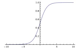 [source: 3]
Tanh
Tanh activation is a scaled version of sigmoid function: $$tanh(x)=2σ(2x)−1tanh(x)=2σ(2x)−1$$ Therefore it is zero centered with range [-1,1]. It still have the problem of killing gradient, but generally it is preferred to sigmoid activation.ReLU
Short for Rectified Linear Units. A popular choice. It threshold upon 0. $$ max (0, x) $$ Comparing to the previous two activation methods, it’s much quicker to converge and involves much less computation time due to linearity. And it doesn’t have the issue of non-zero centered. However, it should be noted, if the learning rate is set to be high, part of the neurons will “die” - they will be not activated during the whole training phase. With the learning rate set to be smaller, it won’t be much an issue.SoftMax
A very common choice for multi-class output activation.
Batch Normalization Layer
Batch normalization is a common practice in deep learning. In machine learning tasks, scaling with zero mean and one standard deviation will make the performance better. However, in deep learning, even if we normalize the data at the very beginning, the data distribution will change a lot in deeper layers. Therefore with batch normalization layer, we could always do data preprocessing again. It is often used right after the fully connected layer or convolutional layer, before the non-linear layers. It makes a significant difference and becomes much more robust to bad initializations.
Drop Out Layer
Drop out layer is a common choice to prevent over fitting. It’s fast and effective. It will keep some neurons activated or 0 according to probabilities.
Convolutional Layer
Convolutional layer produces output with image kernels. Basically it will produce dot product for the image kernel and a sliding window of the input. One 3-D demonstration for the convolutional layers could be found here and computational demo could be found here.
Pooling Layer
Pooling layer is often used after convolutional layer for down sampling. It reduces the amount of parameters carried forward while retaining the most useful information; thus it also prevents overfitting. A demonstration for max pooling could be shown in following picture: 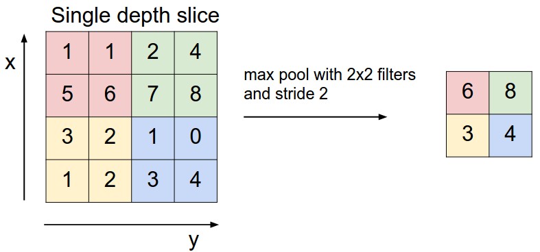 [source: 3]
Sample Architecture and Codes
Sample architecture for convolutional neural network is as follows:
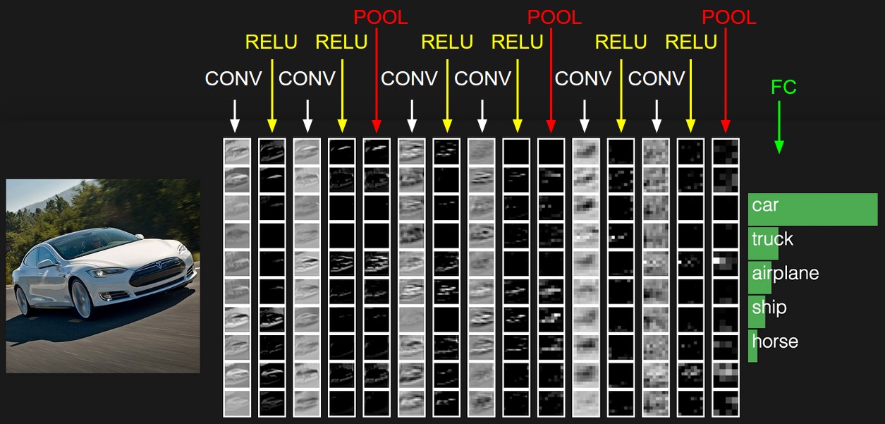 [source: 3]
Sample codes for MNIST solution using keras deep learning as follows:
|
|
code source: keras documentation